Getting started
This page briefly explains how to get started with FramAT. The goal is to give you a basic understanding of how FramAT works, and how analyses can be set up and run. We also explain how to fetch result data which may be of interest to you. Please note that the model interface and all available model and result parameters are explained in more detail on the following pages.
Python API
FramAT provides a pure Python interface which allows you to set up a beam model in a simple Python script. Therefore, some some basic Python knowledge is assumed, but no advanced skills are needed.
Built-in models
FramAT includes a number of built-in models which allows you to run a full beam analysis with only a few lines of code. The simplest model is a single cantilever beam loaded with a point load at the free end. First, create a Python script (or download the script from the link below) and run it with python example_cantilever.py.
Download: example_cantilever.py
from framat import Model                  # Import the FramAT model object

model = Model.from_example('cantilever')  # Load the cantilever example model
model.run()                               # Run the pre-defined analysis
When running the script from a terminal you should see a few log entries providing feedback about the program status, and an interactive plot should be created displaying the beam model.
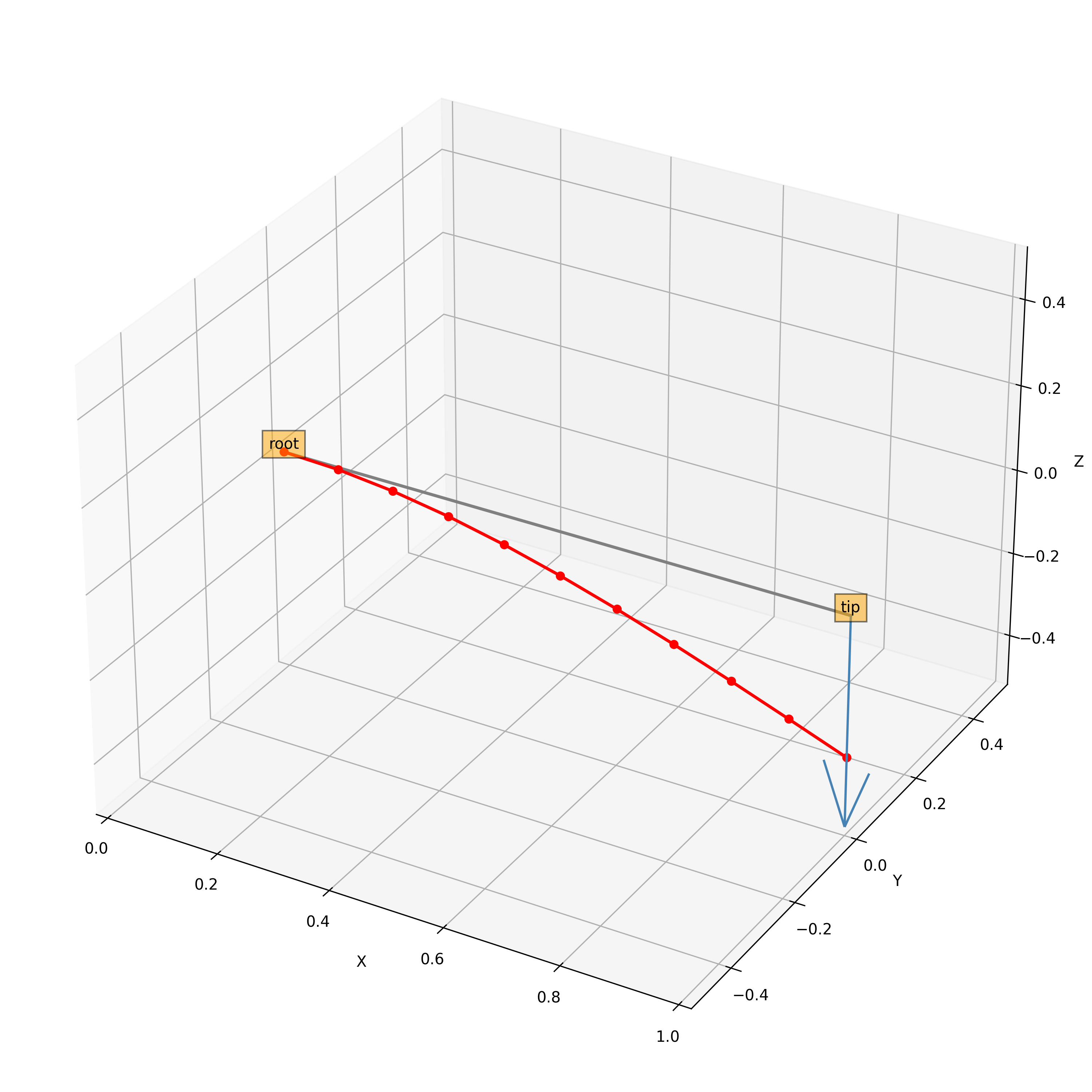
Fig. 2 Simple built-in cantilever model
This example is, admittedly, not the most exciting model, but it allows you to easily check that FramAT has been installed correctly on your system and works. Note that you can try to run some other (perhaps more exciting) built-in models. Just replace 'cantilever' with one of the following strings.
- Built-in models
'cantilever''helix'
Building your own model
Now, let’s explore a few more options to give you an overview of how to actually set up and run your own model. We do not go through all features that are available to you. We only show the most basic features, but if you understand the following example you will be able to easily make use of the other features which are documented on the next pages. As with the previous example we highly encourage you to try it out yourself. Just download the script and run it. Make sure to read the comments in the script and play around with the script to get a feel for how FramAT works.
Download: example_model2.py
# The Model object is used to set up the entire structure model, and to run a
# beam analysis
from framat import Model

# Create a new instance of the Model object
model = Model()

# ===== MATERIAL =====
# Create a material definition which can be referenced when creating beams.
# Note that you can add as many materials as you want. Just provide a different
# UID (unique identifier) for each new material. Below we define the Young's
# modulus, the shear modulus and the density.
mat = model.add_feature('material', uid='dummy')
mat.set('E', 1)
mat.set('G', 1)
mat.set('rho', 1)

# ===== CROSS SECTION =====
# Besides material data, we also need cross section geometry, or more
# specifically, the cross section area, the second moments of area, and the
# torsional constant.
cs = model.add_feature('cross_section', uid='dummy')
cs.set('A', 1)
cs.set('Iy', 1)
cs.set('Iz', 1)
cs.set('J', 1)

# ===== BEAM =====
# Next, let's add a beam! We define the geometry using "named nodes", that is,
# we provide the coordinates of some "support nodes" which can be referred to
# with their UIDs.
beam = model.add_feature('beam')
beam.add('node', [0.0, 0, 0], uid='a')
beam.add('node', [1.5, 0, 0], uid='b')
beam.add('node', [1.5, 3, 0], uid='c')
beam.add('node', [0.0, 3, 0], uid='d')
# Set the number of elements for the beam.
beam.set('nelem', 40)
# Set the material, cross section and cross section orientation
beam.add('material', {'from': 'a', 'to': 'd', 'uid': 'dummy'})
beam.add('cross_section', {'from': 'a', 'to': 'd', 'uid': 'dummy'})
beam.add('orientation', {'from': 'a', 'to': 'd', 'up': [0, 0, 1]})
# Add some line loads [N/m] and point loads [N]
beam.add('distr_load', {'from': 'a', 'to': 'b', 'load': [0, 0, -2, 0, 0, 0]})
beam.add('distr_load', {'from': 'c', 'to': 'd', 'load': [0, 0, -2, 0, 0, 0]})
beam.add('distr_load', {'from': 'b', 'to': 'c', 'load': [0, 0, 1, 0, 0, 0]})
beam.add('point_load', {'at': 'b', 'load': [+0.1, +0.2, +0.3, 0, 0, 0]})
beam.add('point_load', {'at': 'c', 'load': [-0.1, -0.2, -0.3, 0, 0, 0]})

# ===== BOUNDARY CONDITIONS =====
# We also must constrain our model. Below, we fix the nodes 'a' and 'd'
bc = model.set_feature('bc')
bc.add('fix', {'node': 'a', 'fix': ['all']})
bc.add('fix', {'node': 'd', 'fix': ['all']})

# ===== POST-PROCESSING =====
# By default the analysis is run without any GUI, but to get a visual
# representation of the results we can create a plot
pp = model.set_feature('post_proc')
pp.set('plot_settings', {'show': True})
pp.add('plot', ['undeformed', 'deformed', 'node_uids', 'nodes', 'forces'])

# Run the beam analysis
results = model.run()

# ===== RESULTS =====
# The result object contains all relevant results. For instance, we may fetch
# the global load vector.
load_vector = results.get('tensors').get('F')
print(load_vector)
...
When running the script above you should the following plot.
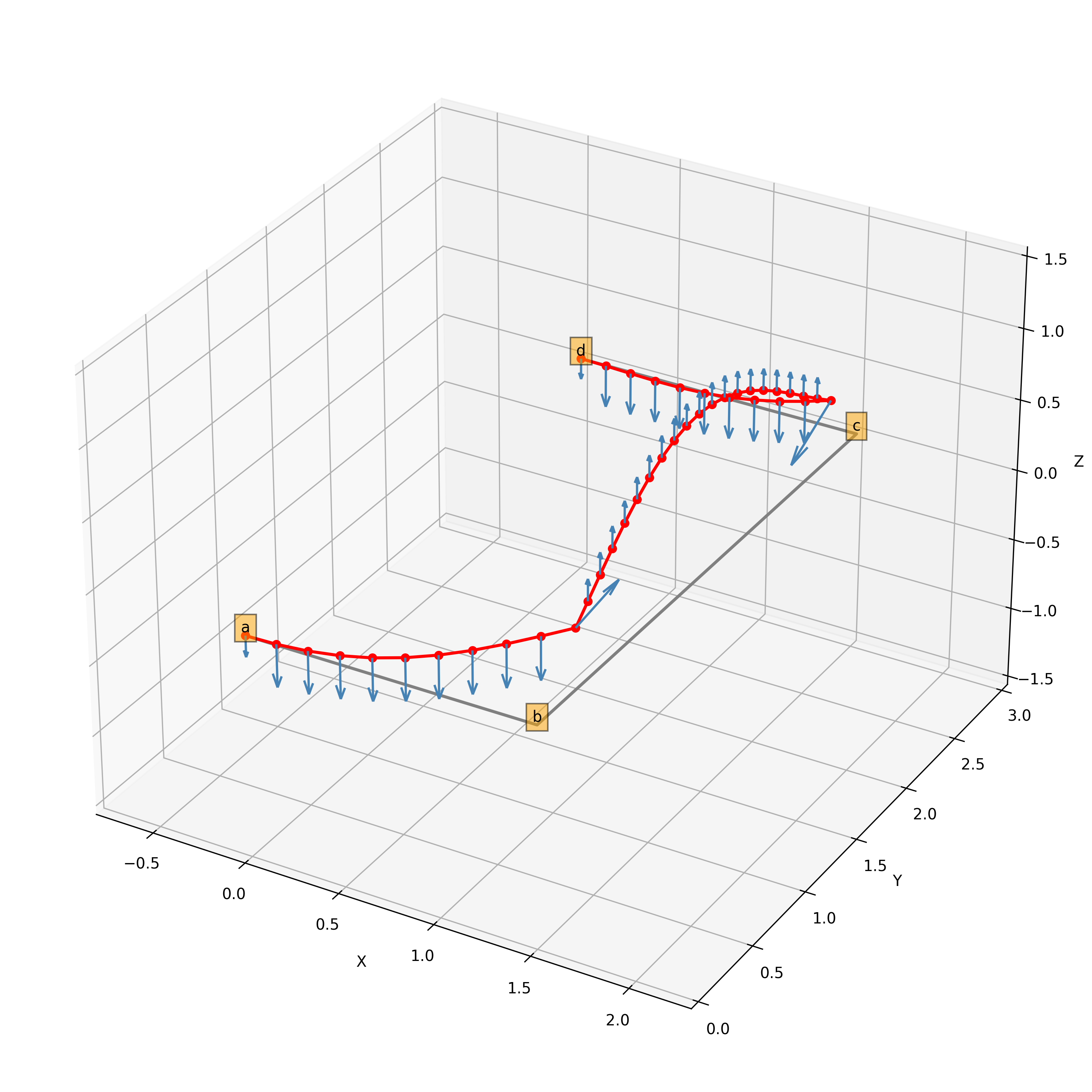
Fig. 3 Example model
Fetching result data
Whenever you perform a new analysis, you will use the model.run() method. This function will always return a results object which behaves very much like the model object itself. All available result data is fully documented on the following pages.